Beethoven's metronome from photographs
from Conductors’ tempo choices shed light over Beethoven’s metronome
Almudena Martín-Castro, Iñaki Ucar
2020-12-16
Source:vignettes/metr-model.Rmd
metr-model.RmdThis vignette discusses and validates a mathematical model using experimental measurements from a contemporary metronome (see help(metr.data)). Then, we fit the metronome model for several metronomes to obtain their nondimensionalized masses, and finally, we characterize Beethoven’s metronome.

Mechanical metronomes. From left to right, a contemporary Neewer© NW-707, TB 06, TB 07 (both from Tony Bingham’s Metronomes and Musical Time), Maelzel’s patent, and a diagram depicting the main parameters of the model.
The model
Contemporary mechanical metronomes preserve essentially the same design as Maelzel’s metronome. The angular frequency of oscillation, \(\Omega\), is obtained as a function of three multiplicative terms:
\[ \Omega = f_\mathrm{ang}^{-1}(\theta)\cdot f_\mathrm{fric}^{-1}(\epsilon)\cdot \sqrt[]{g\frac{M'R -\frac{\mu'}{2} (l-L) -r}{M'R^2 + \frac{\mu'}{3} ( L^2 + l^2- lL) + r^2}} \]
where the last term draws from the classical expression for an ideal double pendulum, but includes corrections to account for the effect in the moment of inertia of the non-negligible mass, \(\mu\), of the rod. Other parameters are the gravitational acceleration (\(g\)), the nondimensionalized lower (\(M' = M / m\)) and rod (\(μ' = μ / m\)) masses, the distances of the lower and upper masses to the shaft (\(R\) and \(r\), respectively), and the length of the two ends of the rod from the shaft (\(L\) and \(l\), respectively). The first two terms, \(f_\mathrm{ang}\) and \(f_\mathrm{fric}\), are further corrections to account, respectively, for large oscillations (usually ranging from \(θ = 40°\) to \(60°\)) and friction and impulse forces:
\[ f_\mathrm{ang} (\theta)= 1 + \sum_{n=1}^\infty\left[ \frac{(2n-1)!!}{(2n)!!}\sin^{2n}\left( \frac{\theta}{2} \right) \right]^2\\ f_\mathrm{fric} (\epsilon)= 1 + \frac{1}{\pi}\sin^{-1}\left(\frac{\epsilon}{1-\epsilon}\right) - \frac{1}{\pi} \sin^{-1}\left(\frac{\epsilon}{1+\epsilon}\right) \]
where \(\epsilon = \frac{\tau_\mathrm{roz}}{\Omega^2 I \theta}\) is a nondimensional parameter that must range from \(0 \leq \epsilon \leq 0.5\), so that the equation has a real solution. It is proportional to the friction torque \(\tau\), and inversely proportional to the angular frequency squared and the moment of inertia.
Measurements
A contemporary metronome was used to validate the model. First, the angular frequency for each metronome mark was measured by means of extracting the tickling period over 15-second audio samples. This package contains a sample file with the audio recorded for 100 bpm. These are the steps to measure the frequency:
- Normalize and square the signal.
- Remove noise (just zeroing values under 0.5).
- Find peaks with a sensitivity of 50 ms (see
help(find_peaks)). - Compute the differences (in samples) and transform.
With the sample file:
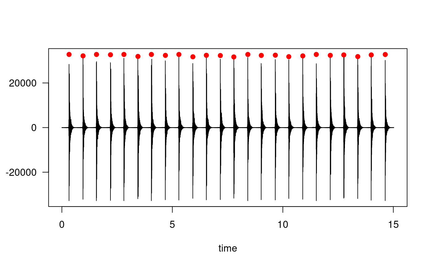
Peak detection in sample file.
f.raw <- tuneR::readWave("100.wav")
f <- tuneR::normalize(f.raw)^2
f@left[f@left < 0.5] <- 0
peaks <- find_peaks(f@left, f@samp.rate * 0.05)

tuneR::plot(f.raw)
points(peaks/f@samp.rate, abs(f.raw@left[peaks]), col="red", pch=19)
period <- diff(peaks) / f@samp.rate
set_errors(60) / set_errors(mean(period), sd(period)/sqrt(length(period)))
## 96.4(4)The same procedure was repeated with all the files:
wav <- Sys.glob(paste0(PATH_WAVS, "/*"))
mark <- as.numeric(sub(".wav", "", basename(wav)))

bpm <- do.call(c, lapply(wav, function(x) {
  f <- tuneR::normalize(tuneR::readWave(x))^2
  f@left[f@left < 0.5] <- 0
  peaks <- find_peaks(f@left, f@samp.rate * 0.05)
  period <- diff(peaks) / f@samp.rate
  set_errors(60) / set_errors(mean(period), sd(period)/sqrt(length(period)))
}))
All these measurements are included in the metr.neewer data set:
head(metr.neewer)## mark bpm bpm.se
## 1 40 37.65203 0.6741290
## 2 42 39.50508 0.6750543
## 3 44 41.97662 0.6010792
## 4 46 44.11887 0.5014112
## 5 48 45.99899 0.5032427
## 6 50 47.88837 0.5011762Model accuracy
Then, the metronome was dismantled and all model parameters were measured (dimensions and masses). Our model achieves even better accuracy than the calibration set by the manufacturer (MAE of less than 2 bpm, compared to a MAE of 3 bpm for the metronome scale).
# measurements for the masses
# M <- set_errors(30.8, 0.01)
# mu <- set_errors(3.8, 0.01)

# correction for L = R, as for the rest of the metronomes
metr.params[1,]$L <- metr.params[1,]$R
M <- set_errors(31.01, 0.01)
m <- set_errors(7.1, 0.01)
mu <- set_errors(3.59, 0.01)
M. <- M / m
mu. <- mu / m

# gravitational acceleration
g <- set_errors(9.807, 0.04)

# attach rcm, l, R, L, A
metr.params %>%
  filter(model == "Neewer") %>%
  unite_errors() %>%
  attach()

neewer <- metr.marks %>%
  filter(model == "Neewer") %>%
  left_join(metr.neewer, by="mark") %>%
  unite_errors()

comparative <- neewer %>%
  mutate(Model  = metr_model(r+rcm, R, M., l, L, mu., g, A)) %>%
  mutate(Forsen = metr_model(r+rcm, R, M., l, L, 0,   g, 0)) %>%
  gather_errors("series", "value", "Model", "Forsen", "bpm") %>%
  mutate(series = sub("Forsen", "Forsén et al. (2013)", series)) %>%
  mutate(series = sub("bpm", "Experimental", series)) %>%
  mutate(series = reorder(factor(series), -drop_errors(value)))

ggplot(comparative) +
  aes(mark, drop_errors(value), color=series) +
  ggthemes::geom_rangeframe(aes(y=drop_errors(bpm)), data=neewer, color="black") +
  geom_abline(slope=1, color="gray") + geom_point(size=.7) +
  geom_errorbar(aes(ymin=errors_min(value), ymax=errors_max(value)), size=.3) +
  geom_smooth(method="gam", size=.3) +
  labs(x="Metronome mark [bpm]", y="Oscillation frequency [bpm]", color=NULL) +
  theme(legend.position=c(0, 1), legend.justification=c(0, 1),
        axis.title.y=element_text(hjust=0.2), axis.title.x=element_text(hjust=0.5))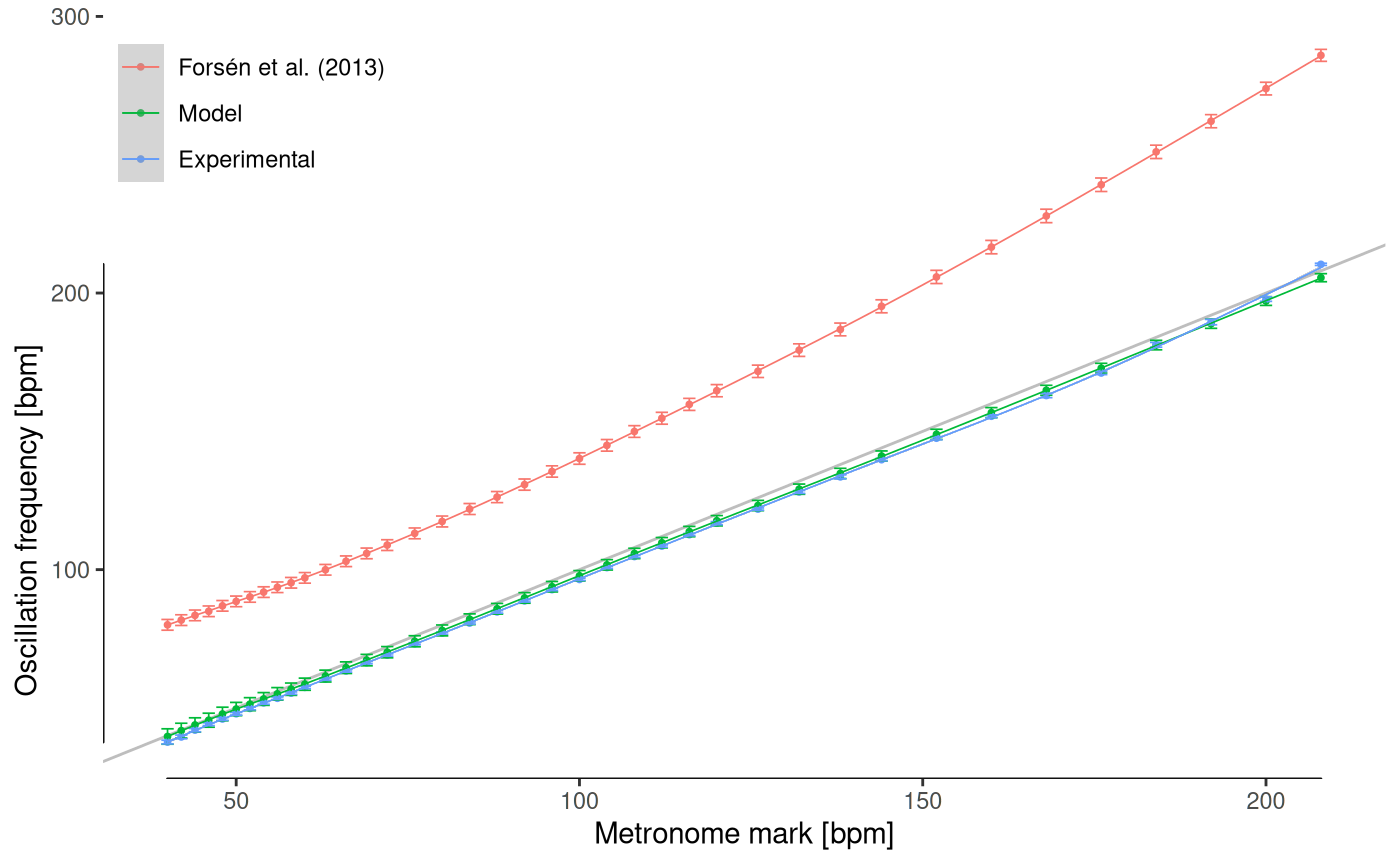
Model validation. The parametrization of a contemporary metronome is compared to its experimental oscillation frequency. It should be noted that the experimental results do not exactly follow the 1:1 relation (gray line), which means that the calibration of the scale has a small error, and our model accurately predicts it. The model by Forsén et al. (2013), which uses a double pendulum without corrections, is included for completeness.
Effect of corrections
The same contemporary metronome was used to study the effect of each kind of correction. To this end, the true mass of the rod, the true oscillation angle and the maximum friction allowed by the model (\(\epsilon = 0.5\)) were separately compared against the null model (null mass, oscillation angle and friction) along the whole scale range.
corrections <- neewer %>%
  mutate(base     = metr_model(r+rcm, R, M., l, L, 0,   g, 0, 0)) %>%
  mutate(Rod      = metr_model(r+rcm, R, M., l, L, mu., g, 0, 0)) %>%
  mutate(Angle    = metr_model(r+rcm, R, M., l, L, 0,   g, A, 0)) %>%
  mutate(Friction = metr_model(r+rcm, R, M., l, L, 0,   g, 0, 0.5)) %>%
  mutate(Rod      = (Rod      - base) / base * 100) %>%
  mutate(Angle    = (Angle    - base) / base * 100) %>%
  mutate(Friction = (Friction - base) / base * 100) %>%
  gather_errors("series", "value", "Rod", "Angle", "Friction") %>%
  mutate(series = factor(series, levels=c("Friction", "Angle", "Rod")))

ggplot(corrections) +
  aes(mark, drop_errors(value), color=series) +
  ggthemes::geom_rangeframe(color="black") +
  geom_point(size=.7) +
  geom_errorbar(aes(ymin=errors_min(value), ymax=errors_max(value)), size=.3) +
  geom_smooth(method="gam", size=.3) +
  labs(x="Metronome mark [bpm]", y="Correction [%]", color="") +
  theme(legend.position=c(0.98, 0.58), legend.justification=c(1, 0))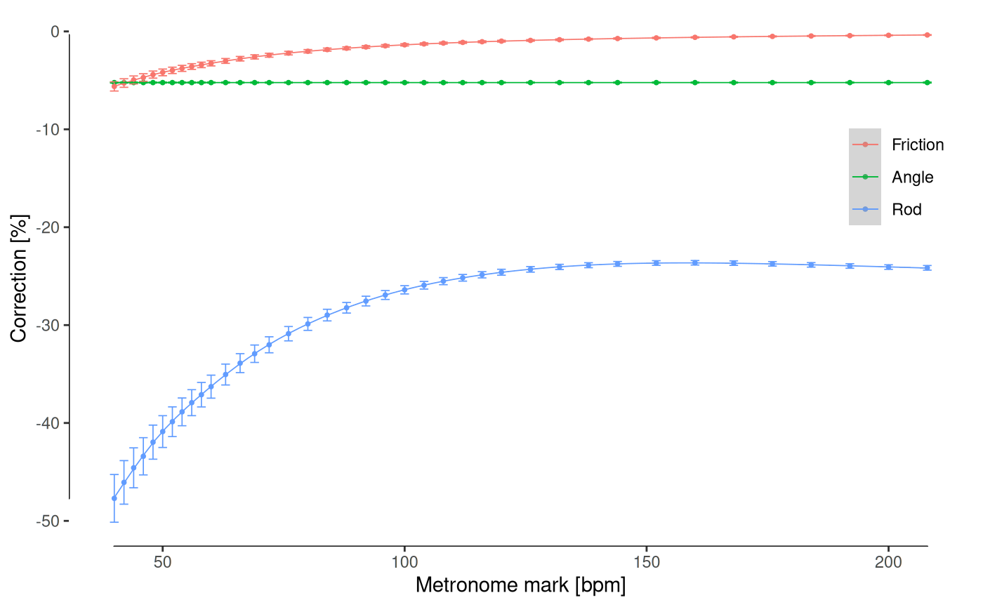
Effect of corrections throughout the whole range for the same metronome, expressed as a percentage over the null model (frictionless, small-angle approximation for a massless rod) for each metronome mark.
As expected, considering the mass of the rod contributes the most to the model accuracy, and thanks to the escapement wheel, the effect of friction is negligible except for the lowest oscillation frequencies.
Model transformation and fit
Neglecting the effect of friction (\(f_\mathrm{fric} \approx 1\)), we express \(\Omega^2\) as a linear combination of polynomial terms of \(r\):
\[ \Omega^2=a_0 + b_2 \left(\frac{g}{f_\mathrm{ang}^2(\theta)} r + \Omega^2 r^2 \right) \]
where
\[ a_0= \frac{g}{f_\mathrm{ang}^2(\theta)} \cdot \frac{M'R-\frac{\mu'}{2}(l-L)}{M'R^2+\frac{\mu'}{3}(L^2+l^2-lL)} \\ b_2= -\frac{1}{M'R^2+\frac{\mu'}{3}(L^2+l^2-lL)} \]
Results
This linear model was fitted for two old metronomes from dates similar to Beethoven’s metronome, the patent diagram, and the contemporary metronome as a control (see first figure).
metr <- metr.marks
metr[grep("Neewer", metr$model),]$mark <- rep(metr.neewer$bpm, 2)
metr <- metr %>%
  group_by(model) %>%
  slice(-n())

fit <- metr_fit(metr, metr.params) %>%
  unite_errors() %>%
  mutate(model = factor(sub("Neewer", "Control", model)))

pred <- metr_predict(fit) %>%
  cbind(metr[-1]) %>%
  unite_errors() %>%
  mutate(model = factor(sub("Neewer", "Control", model)))

r.squared <- sapply(fit$fit, function(x) summary(x)$adj.r.squared)
labels <- mapply(function(x, y) {
  bquote(.(x)*"," ~ R^2==.(y))
}, levels(pred$model), round(r.squared, 4))

ggplot(pred) +
  aes(drop_errors(r), y, color=reorder(model, drop_errors(r), min)) +
  ggthemes::geom_rangeframe(color="black") +
  geom_ribbon(aes(ymin=lwr, ymax=upr), alpha=.2, size=0) +
  geom_point(size=.7) +
  geom_errorbarh(aes(xmin=errors_min(r), xmax=errors_max(r)), height=2, size=.3) +
  geom_line(aes(y=fit), size=.3) +
  scale_color_discrete(labels=labels) +
  labs(x="r [mm]", y=expression(Omega^2), color=NULL) +
  theme(legend.position=c(1, 1), legend.justification=c(1, 1))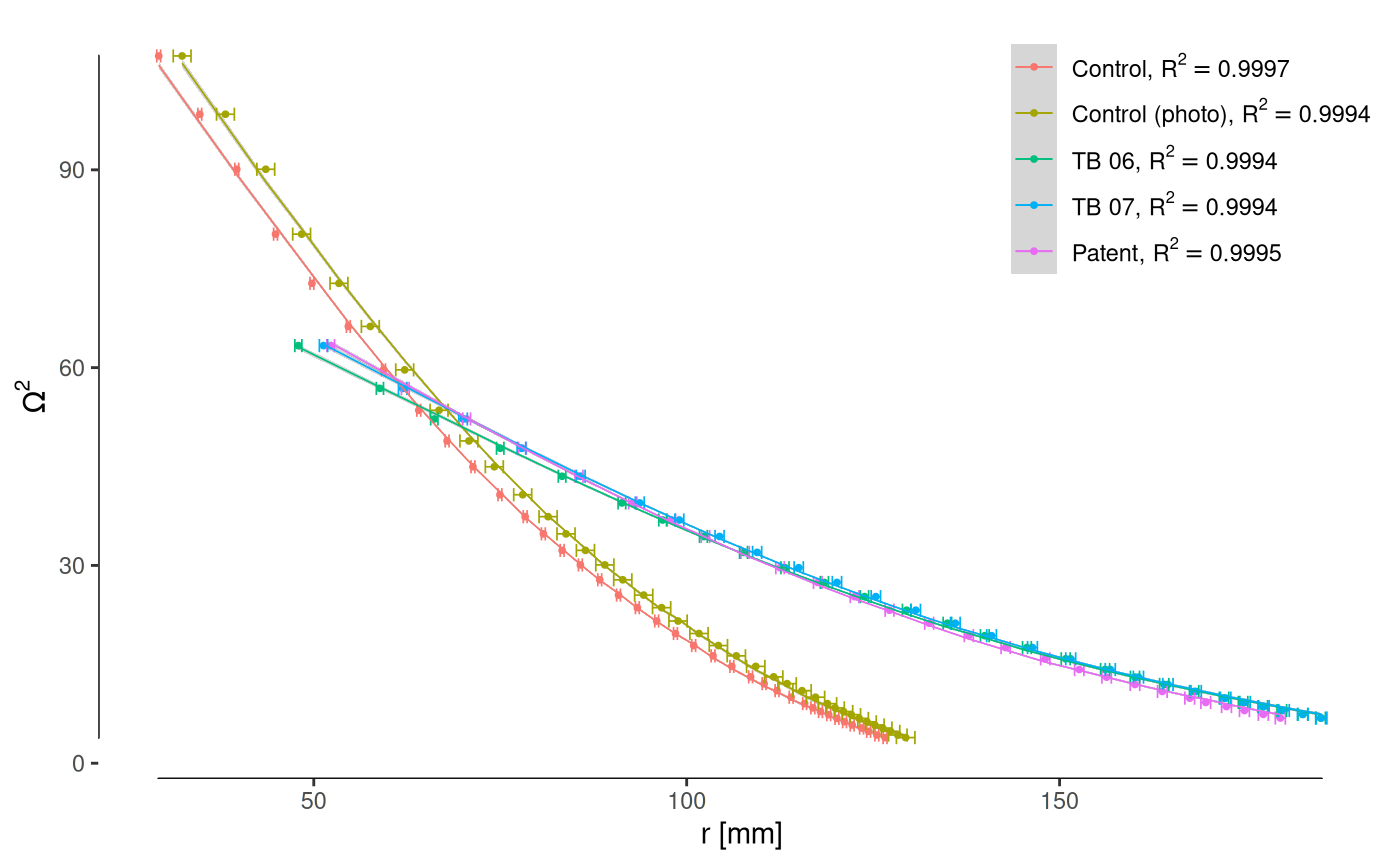
Model fit for the oscillation frequency squared as a function of the position of the moving weight.
Metronome dimensions were measured using Fiji on the basis of the total heights reported in Tony Bingham’s catalogue. The total height is assumed to be 31 cm for the patent according to the patent description and the height of the oldest metronome. The oscillation angle is taken as the maximum inclination, bounded by the box. Parameter R cannot be directly measured for some metronomes (when the box hides the lower mass), so it was estimated taking into account the box size and the patent description. Given that the lower mass hangs approximately from the end of the rod, it is assumed that \(L \approx R\). With these assumptions, we estimated the nondimensional masses, \(M'\) and \(μ'\), for each metronome from the regression coefficients.
note <- data.frame(model="Control (true)", M.=M., mu.=mu.)

ggplot(fit) +
  aes(drop_errors(M.), drop_errors(mu.), color=reorder(model, -drop_errors(mu.))) +
  ggthemes::geom_rangeframe(color="black") +
  geom_point(size=.7) +
  geom_point(aes(shape=model), data=note, color="black", size=2) +
  geom_errorbarh(aes(xmin=errors_min(M.), xmax=errors_max(M.)), height=.005, size=.3) +
  geom_errorbar(aes(ymin=errors_min(mu.), ymax=errors_max(mu.)), width=.012, size=.3) +
  scale_shape_manual(name=NULL, values=8) +
  labs(x="Nondimensionalized lower mass", y="Nondimensionalized rod mass", color=NULL) +
  guides(color=guide_legend(order=1), shape=guide_legend(order=2)) +
  theme(legend.position=c(.95, .95), legend.justification=c(1, 1), legend.spacing.y=unit(-2, "mm"))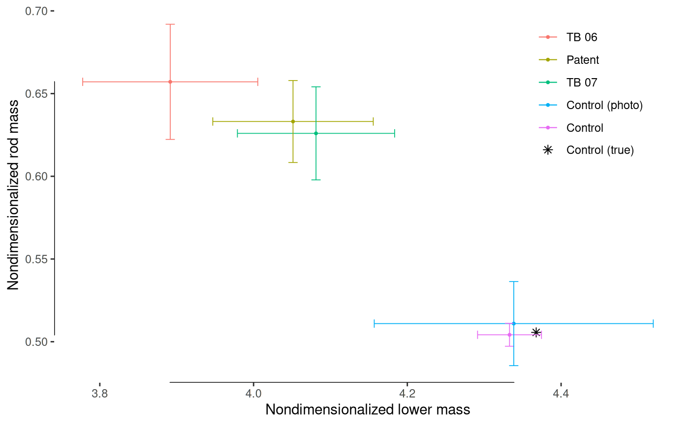
Parameter estimation for all the metronomes considered. Estimation of nondimensionalized masses \(\mu'\) (rod) and \(M'\) (lower mass). Both controls (measuring a dismantled metronome with precision as well as measuring all the distances from a photograph) accurately estimate the true masses for the contemporary metronome, thus validating the estimation for the rest of the metronomes.
Beethoven’s metronome
Results show that this methodology accurately estimates the masses for the control metronome, and thus, we take the averages of the old metronomes and the patent as a parametrization of Beethoven’s metronome, with the rest of the parameters equal to the measurements for the patent.
res <- as.data.frame(fit[3:5, 1:3])
res$model <- as.character(res$model)
res[4,] <- list("Beethoven's metronome (average)", mean(res$M.), mean(res$mu.))
knitr::kable(res, caption=table1)| model | M. | mu. |
|---|---|---|
| Patent | 4.1(1) | 0.63(2) |
| TB 06 | 3.9(1) | 0.66(3) |
| TB 07 | 4.1(1) | 0.63(3) |
| Beethoven’s metronome (average) | 4.0(1) | 0.64(3) |