7 Performance of RA-TPC Algorithms in 802.11
So far, we have demonstrated through numerical analysis, and validated experimentally47, the existence of a trade-off between two competing performance figures, namely, goodput and energy efficiency. This issue arises even for a single spatial stream in absence of interference. Furthermore, we have discussed in Section 6.3.2 some ideas about the kind of mechanisms that energy-aware RA-TPC algorithms may incorporate, to leverage the behaviour that we have identified in our analysis in these so-called mode transitions. Summing up, the algorithms should be conservative during these transitions.
During that discussion, we neglected the challenge of estimating channel conditions. But in practice, any RA-TPC algorithm has imperfect channel knowledge, and therefore will adapt to changing conditions in a suboptimal way. In this chapter, we will analyse and compare the performance of several representative existing RA algorithms, which also incorporate TPC, to confirm whether the conservativeness in such decisions may have a positive impact on the achieved performance.
In the following, we first present the algorithms considered and describe a simple simulation scenario to test them. Our results will lead us to a more detailed discussion about conservativeness at mode transitions.
7.1 Algorithms Considered
If we take a look at the actual operation of WiFi networks, the Minstrel (Mcgregor and Smithies 2017) algorithm, which was integrated into the Linux kernel, has become the de facto standard due to its relatively good performance and robustness. However, Minstrel does not consider TPC and, in consequence, there is no TPC in today’s WiFi deployments. Moreover, despite some promising proposals have been presented in the literature, there are very few of them implemented, although there are some ongoing efforts such as the work by the authors of Minstrel-Piano (Huehn and Sengul 2012), who are pushing to release an enhanced version of the latter for the Linux kernel with the goal of promoting it upstream.48
As already stated, RA is a very prolific research line in the literature, but the main corpus is dedicated to the MCS adjustment without taking into account the TXP49. There is some work considering TPC, but the motivation is typically the performance degradation due to network densification, and the aim is interference mitigation and not energy efficiency. Given that we are interested in assessing RA implementations with TPC support, we consider only open-source algorithms that can be tested using the NS-3 Network Simulator50. After a thorough analysis of the literature, we considered the following set of algorithms:
- Power-controlled Auto Rate Fallback
- (PARF), (Akella et al. 2005) which is based on Auto Rate Fallback (ARF) (Ad Kamerman and Monteban 1997), one of the earliest RA schemes for 802.11. ARF rate adaptation is based on the frame loss ratio. It tunes the MCS in a very straightforward and intuitive way. The procedure starts with the lowest possible MCS. Then, if either a timer expires or the number of consecutive successful transmissions reach a threshold, the MCS is increased and the timer is reset. The MCS is decreased if either the first transmission at a new rate fails or two consecutive transmissions fail. PARF builds on ARF and tries to reduce the TXP if there is no loss until a minimum threshold is reached or until transmissions start to fail. If transmission fails persist, the TXP is increased.
- Minstrel-Piano
- (MP) (Huehn and Sengul 2012) is based on Minstrel (Mcgregor and Smithies 2017). Minstrel performs per-frame rate adaptation based on throughput. It randomly probes the MCS space and computes an exponential weighted moving average (EWMA) on the transmission probability for each rate, in order to keep a long-term history of the channel state. As the previous algorithm, MP adds TPC without interfering with the normal operation of Minstrel. It incorporates to the TPC the same concepts and techniques than Minstrel uses for the MCS adjustment, i.e., it tries to learn the impact of the TXP on the achieved throughput.
- Robust Rate and Power Adaptation Algorithm
- (RRPAA) and Power, Rate and Carrier-Sense Control (PRCS), (Richart, Visca, and Baliosian 2015) which are based on Robust Rate Adaptation Algorithm (RRAA) (Wong et al. 2006). RRAA consists of two functional blocks, namely, rate adaptation and collisions elimination. It performs rate adaptation based on loss ratio estimation over short windows, and reduces collisions with a RTS-based strategy. The procedure starts at the maximum MCS. The loss ratio for each window of transmissions is available for rate adjustment in the next window. There are two thresholds involved in this adjustment: if the loss ratio is below both of them, the MCS is increased; if it is above, the MCS is decreased; and if it is in between, the MCS remains unchanged. RRPAA and PRCS build on this and try to use the lowest possible TXP without degrading the throughput. For this purpose, they firstly find the best MCS at the maximum TXP and, from there, they jointly adjust the MCS and TXP for each window based on a similar thresholding system. RRPAA and PRCS are very similar and only differ in implementation details.
Based on their behaviour, these algorithms can be classified into three distinct classes. First of all, MP is the most aggressive technique, given that it constantly samples the whole MCS/TXP space searching for the best possible configuration. On the opposite end, RRPAA and PRCS do not sample the whole MCS/TXP space. Instead, they are based on a windowed estimation of the loss ratio, which makes the MCS/TXP transitions much lazier. Finally, PARF falls in between, as it changes the MCS/TXP to the next available proactively if a number of transmissions are successful, but it falls back to the previous one if the new one fails. In practice, this may result in some instability during transitions.
7.2 Simulation Scenario
This evaluation is publicly available,51 and builds upon the code provided by Richart, Visca, and Baliosian (2015)52. We assessed the proposed algorithms in the toy scenario depicted in Figure 7.1. It consists of a single access point (AP) and a single mobile node connected to this AP configured with the 802.11a PHY. The mobile node at the farthest distance at which is able to communicate at the lowest possible rate (6 Mbps) and highest TXP (17 dBm), and then it moves at constant speed towards the AP. The simulation stops when the node is directly in front of the AP and it is able to communicate at the highest possible rate (54 Mbps) and lowest TXP (0 dBm). This way, we sweep through all mode transitions available.
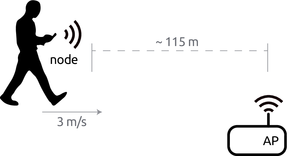
Figure 7.1: Simulation scenario.
For the whole simulation, the AP tries to constantly saturate the channel by sending full-size UDP packets to the node. Every transmission attempt is monitored, as well as every successful transmission. The first part allows us to compute the transmission time, while the latter allows us to compute the reception time (of the ACKs) and the goodput achieved.
The simulation model assembles the power model from Equation (1.1) with the parametrisation previously made (see Table 6.2) for all the devices considered in Section 6.2: HTC Legend, Linksys WRT54G, Raspberry Pi, Samsung Galaxy Note 10.1 and Soekris net4826-48. Thus, the total energy consumed is computed for all the devices and each run using the computed transmission time, reception time and idle time. Beacons are ignored and considered as idle time.
We set up one simulation for each algorithm (PARF, MP, PRCS, RRPAA) with a fixed seed, and perform 10 independent runs for each simulation. We use boxplots to show aggregated results unless otherwise mentioned.
7.3 Results and Discussion
We first analyse the goodput achieved per each algorithm, which are depicted in Figure 7.2. The median of the average goodput across several runs for RRPAA is the highest, followed by PRCS, PARF and MP. PRCS and RRPAA, which are very similar mechanisms, show a higher variability across replications compared to PARF and MP, which have little dispersion.
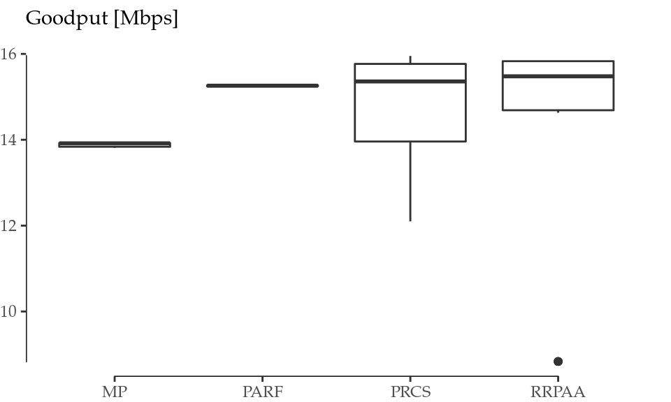
Figure 7.2: Goodput achieved per simulated algorithm.
Figure 7.3 shows the energy efficiency achieved per algorithm, computed for all the devices considered. As expected, the numerical values of the energy efficiency achieved are different across devices, but the relative performance is essentially the same, as in the previous case. Indeed, the efficiency follows the pattern seen in Figure 7.2: RRPAA results the most energy efficient in our scenario, followed by PRCS, PARF and MP. PRCS and RRPAA exhibit the same variability across replications as in the case of goodput, which is particularly notable for the most efficient devices, i.e., the HTC Legend and the Samsung Galaxy Note.
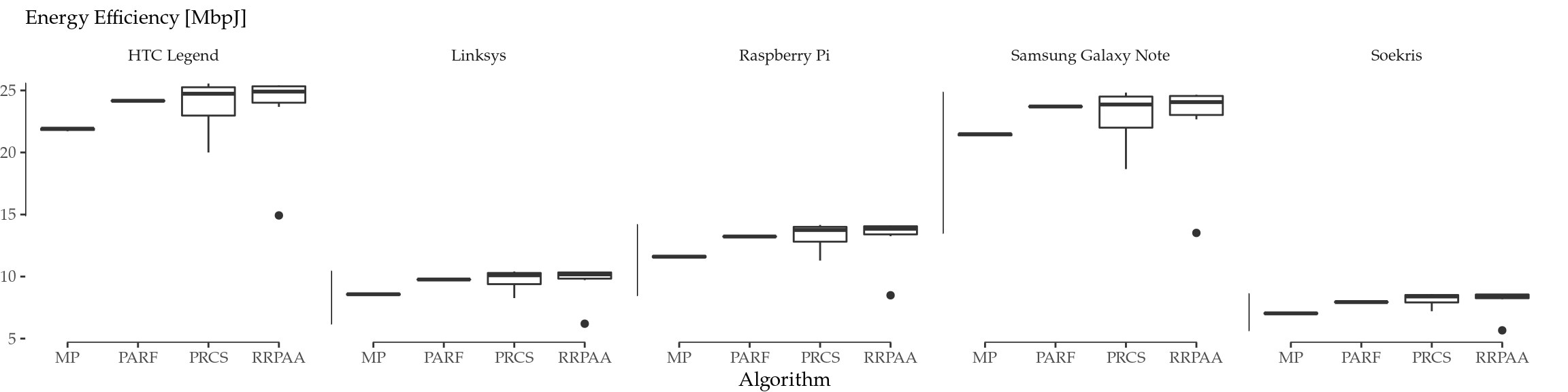
Figure 7.3: Energy efficiency achieved per simulated algorithm and device.
In order to shed some light into the reasons behind the differences in performance, Figures 7.4 show the behaviour of each algorithm throughout the simulation time for one run, showing the evolution of the MCS and TXP chosen by each algorithm, respectively. Here, we can clearly differentiate that there are two kinds of behaviour: while MP and PARF are constantly sampling other MCSs and TXPs, PRCS and RRPAA are much more conservative in that sense, and tend to keep the same configuration for longer periods of time.
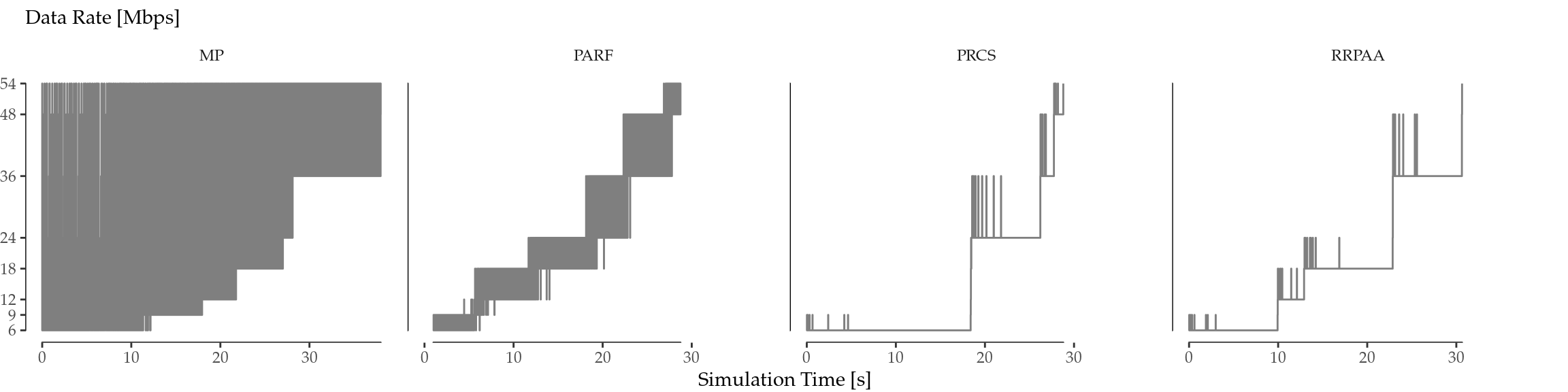
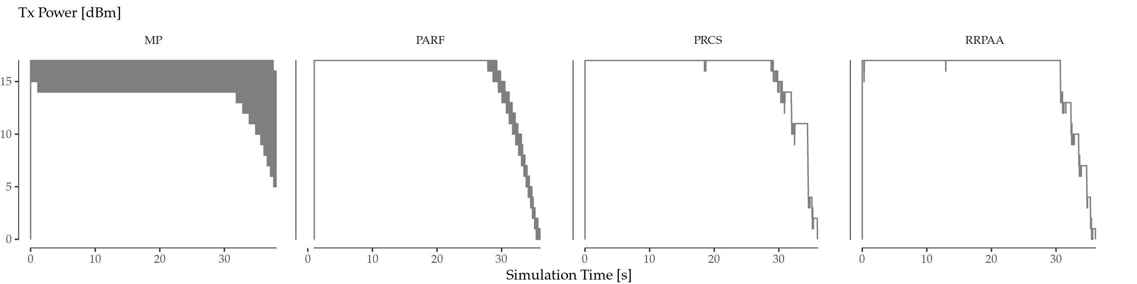
Figure 7.4: MCS (top) and TXP (bottom) evolution per algorithm for a selected run.
MP randomly explores the whole MCS/TXP space above a basic guaranteed value, and this is the explanation for the apparently uniformly greyed zone. Also, this aggressive approach is clearly a disadvantage in the considered toy scenario (deterministic walk, one-to-one, no obstacles), and this is why the achieved goodput in Figure 7.2 is slightly smaller than the one achieved by the others. PARF, on its part, only explores the immediately higher MCS/TXP, which leads to a higher goodput and efficiency.
On the other hand, PRCS and RRPAA sampling is much more sparse in time. As a consequence, Figures 7.4 show more differences across replications, leading to the high variability shown in Figure 7.2 compared to MP and PARF.
In terms of TXP, all the algorithms exhibit a similar aggressiveness, in the sense that they use a high TXP value in general. Indeed, as Figure 7.4 (bottom) shows, the TXP is the highest possible until the very end of the simulation, when the STA is very close to the AP. This is the cause for the high correlation between Figures 7.2 and 7.3.
A noteworthy characteristic of PRCS and RRPAA is that, in general, they delay the MCS change decision, as depicted in Figure 7.4 (top). Most of the times, they do not even use the whole space of MCS available, unlike MP and PARF. Because of this, they tend to achieve the best goodput and energy efficiency.
7.4 Conservativeness at Mode Transitions
Building on the concept of conservativeness (i.e., the tendency to select a lower MCS/TXP in the transition regions), we explore whether there is any correlation with the energy efficiency achieved by a certain algorithm and this tendency. For that purpose, we first define a proper metric.
In the first place, we define the normalised average MCS as the area under the curve in Figure 7.4 (top) normalised by the total simulation time and the maximum MCS:
\[\begin{equation} \widehat{\mathrm{MCS}} = \frac{1}{\max(\mathrm{MCS}) \cdot t_\mathrm{sim}}\int_0^{t_\mathrm{sim}} \mathrm{MCS}(t)dt \tag{7.1} \end{equation}\]
where \(t_\mathrm{sim}\) is the simulation time and \(\max(\mathrm{MCS})\) is 54 Mbps in our case. The same concept can be applied to the TXP:
\[\begin{equation} \widehat{\mathrm{TXP}} = \frac{1}{\max(\mathrm{TXP}) \cdot t_\mathrm{sim}}\int_0^{t_\mathrm{sim}} \mathrm{TXP}(t)dt \tag{7.2} \end{equation}\]
where \(\max(\mathrm{TXP})\) is 17 dBm in our case. Both \(\widehat{\mathrm{MCS}}\) and \(\widehat{\mathrm{TXP}}\) are unitless scores between 0 and 1, and lower values mean a more conservative algorithm. Therefore, we can define a Conservativeness Index (CI) as the inverse of the product of both scores:
\[\begin{equation} \mathrm{CI} = \frac{1}{\widehat{\mathrm{MCS}} \cdot \widehat{\mathrm{TXP}}} \tag{7.3} \end{equation}\]
where \(\mathrm{CI}>1\).
We computed the CI53 for each device and run, and the final results are depicted in Figure 7.5 as the average CI across different runs vs. the median energy efficiency in Figure 7.3.
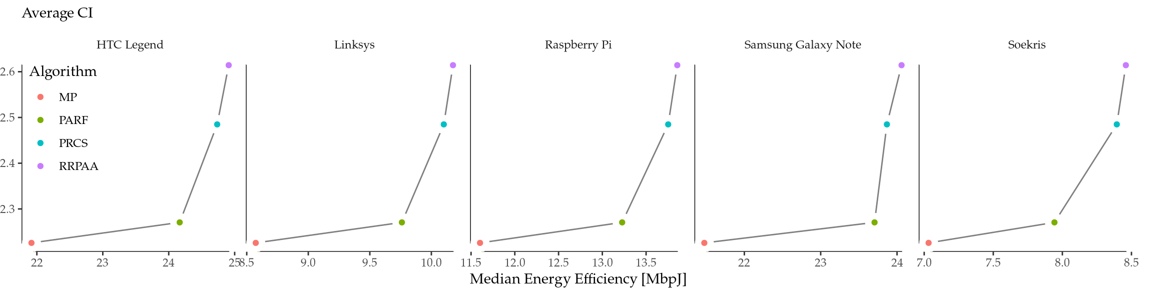
Figure 7.5: Relationship between Conservativeness Index (tendency to select lower MCS and TXP) and energy effienciency per simulated device.
The results in Figure 7.5 show a positive non-linear relationship between the CI of an algorithm and the energy efficiency achieved for all the devices considered. MP is the algorithm with the lowest CI, which is in consonance with its aggressiveness (i.e., frequent jumps between MCS/TXP values, as shown in Figures 7.4, and the goodput achieved was also the lowest, as depicted in Figure 7.2. On the other hand, PARF, PRCS and RRPAA achieved a similar performance in terms of goodput, but the ones with the most conservative behaviour (PRCS and RRPAA, as it can be seen in Figures 7.4) also achieve both the highest CI and energy efficiency.
This result evidences that the performance gaps uncovered by Figure 6.4 under optimal conditions have also an impact in real-world RA-TPC algorithms. Therefore, we confirm that this issue must be taken into account in the design of more energy-efficient rate and transmission power control algorithms.
7.5 Summary
We have extended (Iñaki Ucar, Donato, et al. 2018) our results from Chapter 6 regarding the role of conservativeness at mode transitions in achieving better energy efficiency in RA-TPC algorithms. We have developed a metric to compare algorithms, and we have assessed the performance of four state-of-the-art schemes through simulation. We have demonstrated that certain conservativeness can resolve the trade-off between throughput and energy efficiency optimality, thus making a difference for properly designed energy-aware algorithms.
Further research is needed to develop proper heuristics to leverage these findings. In particular, the downwards direction, as described in Section 6.3.2, is the most challenging, because it requires predicting the evolution of the channel state.
References
Akella, Aditya, Glenn Judd, Srinivasan Seshan, and Peter Steenkiste. 2005. “Self-Management in Chaotic Wireless Deployments.” In Proceedings of the 11th Annual International Conference on Mobile Computing and Networking, 185–99. MobiCom ’05. New York, NY, USA: ACM. https://doi.org/10.1145/1080829.1080849.
Huehn, T., and C. Sengul. 2012. “Practical Power and Rate Control for Wifi.” In 2012 21st International Conference on Computer Communications and Networks (Icccn), 1–7. https://doi.org/10.1109/ICCCN.2012.6289295.
Kamerman, Ad, and Leo Monteban. 1997. “WaveLAN-Ii: A High-Performance Wireless Lan for the Unlicensed Band.” Bell Labs Technical Journal 2 (3). Alcatel-Lucent: 118–33.
Mcgregor, A., and D. Smithies. 2017. “Rate adaptation for 802.11 wireless networks: Minstrel.” http://blog.cerowrt.org/papers/minstrel-sigcomm-final.pdf.
Richart, M., J. Visca, and J. Baliosian. 2015. “Rate, Power and Carrier-Sense Threshold Coordinated Management for High-Density Ieee 802.11 Networks.” In 2015 Ifip/Ieee International Symposium on Integrated Network Management (Im), 139–46. https://doi.org/10.1109/INM.2015.7140286.
Ucar, Iñaki, Carlos Donato, Pablo Serrano, Andres Garcia-Saavedra, Arturo Azcorra, and Albert Banchs. 2018. “On the energy efficiency of rate and transmission power control in 802.11.” Computer Communications 117 (February): 164–74. https://doi.org/10.1016/j.comcom.2017.07.002.
Wong, Starsky H. Y., Hao Yang, Songwu Lu, and Vaduvur Bharghavan. 2006. “Robust Rate Adaptation for 802.11 Wireless Networks.” In Proceedings of the 12th Annual International Conference on Mobile Computing and Networking, 146–57. MobiCom ’06. New York, NY, USA: ACM. https://doi.org/10.1145/1161089.1161107.
It must be taken into account that the CI is not suitable for comparing any algorithm. For instance, in an extreme case, an “algorithm” could select 6 Mbps and 0 dBm always, resulting in a very low CI, but a very bad performance at the same time. The CI should only be used for comparing similarly performant algorithms, as it is the case in our study given the results shown in Figures 7.2 and 7.3.↩