B Experimental Validation of RA-TPC Inefficiencies
This appendix is devoted to experimentally validate the results from the numerical analysis developed in Chapter 6. To this aim, we describe our experimental setup and validation procedure, first specifying the methodology and then the results achieved.
B.1 Experimental Setup
We deployed the testbed illustrated in Figure B.1, which is a variation of the one depicted in Section 3.4, Figure 3.7. It consists of a station (STA) transmitting evenly-spaced maximum-sized UDP packets to an access point (AP), an x86-based Alix6f2 board with a Atheros AR9220 wireless card, running kernel version 3.16.7 and the ath9k driver. The STA is a desktop PC with a Mini PCI Express Qualcomm Atheros QCA9880 wireless network adapter, running Fedora Linux 23 with kernel version 4.2.5 and the ath10k driver58. We also installed at the STA a Mini PCI Qualcomm Atheros AR9220 wireless network adapter to monitor the wireless channel.
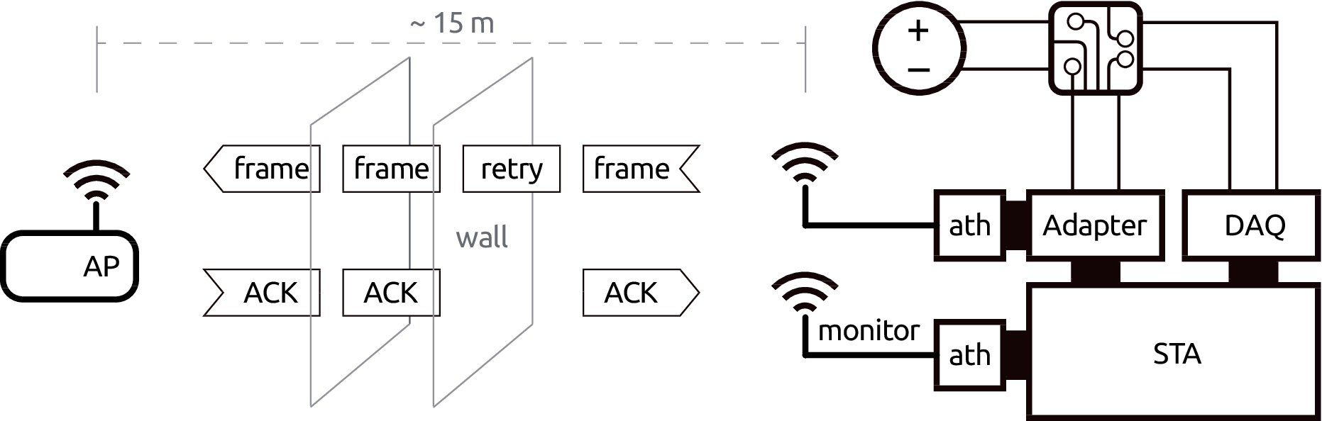
Figure B.1: Experimental setup.
As Figure B.1 illustrates, the STA is located in an office space and the AP is placed in a laboratory 15 m away, and transmitted frames have to transverse two thin brick walls. The wireless card uses only one antenna and a practically-empty channel in the 5-GHz band. Throughout the experiments, the STA is constantly backlogged with data to send to the AP, and measures the throughput obtained by counting the number of acknowledgements (ACKs) received.
B.2 Methodology and Results
In order to validate our results, our aim is to replicate the qualitative behaviour of Figure 6.4, in which there are energy efficiency “drops” as the optimal goodput increases. However, in our experimental setting, channel conditions are not controllable, which introduces a notable variability in the results as it affects both the \(x\)-axis (goodput) and the \(y\)-axis (energy efficiency). To reduce the impact of this variability, we decided to change the variable in the \(x\)-axis from the optimal goodput to the transmission power —a variable that can be directly configured in the wireless card—. In this way, the qualitative behaviour to replicate is the one illustrated in Figure B.2, where we can still identify the performance “drops” causing the loss in energy efficiency.
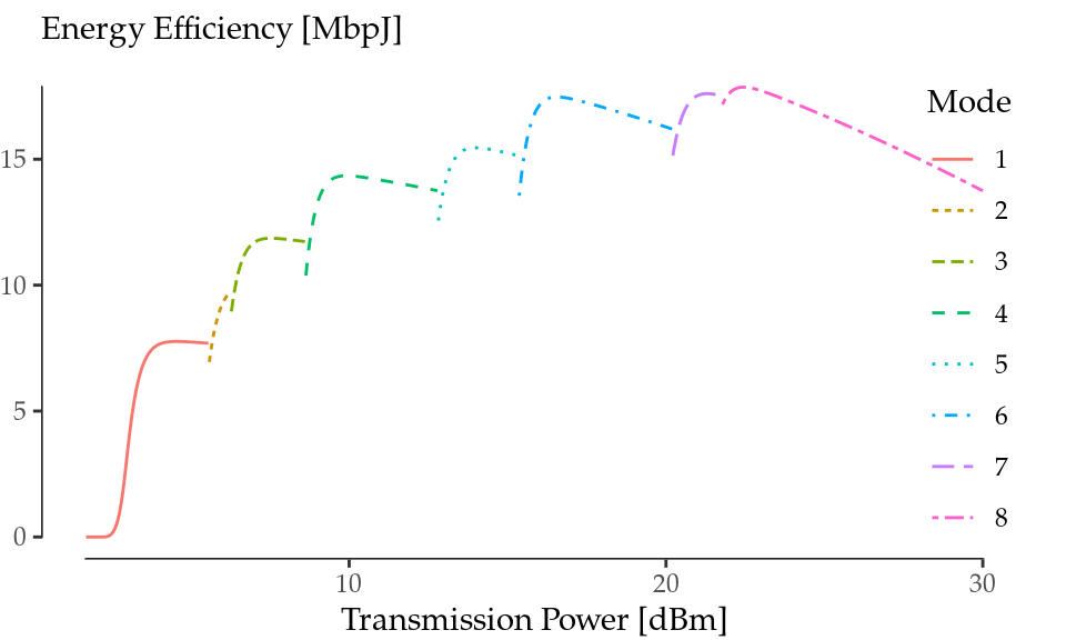
Figure B.2: Energy Efficiency vs. Transmission Power under fixed channel conditions for the Raspberry Pi case.
Building on Figure B.2, we perform a sweep through all available combinations of MCS (see Table 6.1) and TXP.59 Furthermore, we also tested two different configurations of the AP’s TXP at different times of the day, to confirm that this qualitative behaviour is still present under different channel conditions. For each configuration, we performed 2-second experiments in which we measure the total bytes successfully sent and the energy consumed by the QCA9880 card with sub-microsecond precision, and we compute the energy efficiency achieved for each experiment.
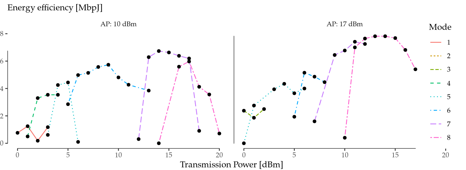
Figure B.3: Experimental study of Figure B.2 for two AP configurations.
The results are shown in Figure B.3. Each graph corresponds to a different TXP value configured at the AP, and depicts a single run (note that we performed several runs throughout the day and found no major qualitative differences across them). Each line type represents the STA’s mode that achieved the highest goodput for each TXP interval, therefore in some cases low modes do not appear because a higher mode achieved a higher goodput. Despite the inherent experimental difficulties, namely, the low granularity of 1-dBm steps and the random variability of the channel, the experimental results validate the analytical ones, as the qualitative behaviour of both graphs follows the one illustrated in Figure B.2. In particular, the performance “drops” of each dominant mode can be clearly observed (especially for the 36, 48 and 54 Mbps MCSs) despite the variability in the results.
Following the discussion on Section 6.3.1 the device’s cross-factor is not involved in the trade-off, thus we will expect to reproduce it by measuring the wireless interface alone.↩
The model explores a range between 0 and 30 dBm to get the big picture, but this particular wireless card only allows us to sweep from 0 to 20 dBm.↩